Easy-peasy Deep Learning and Convolutional Networks with Keras - Part 1

Deep learning… wow… this is “the” hot topic since, at least, some good years ago! I’ve attended a few seminars and workshops about deep learning, nevertheless I’ve never tried to code something myself - until now! - because I had always another priority. Also, I have to admit, I thought it was a lot harder and it would need much more time to be able to run anything that was not simply a sample code.

I’m always forgetting things, so I like to take notes as if I was teaching a toddler. Consequently, this post was designed to remember myself when I forget how to use Keras .

All the things I’ll explain below will only make sense if you know what is a Multilayer perceptron and Feedforward neural network as well. In case you don’t, no worries, Google is your friend .

Since I’ve just learned how to create Github Markdown check boxes, let’s write down an outline of what we want to achieve at the end:

• Convince ourselves learning Keras is a nice investment!
• Create our very own first deep neural network (ok, not that deep) applying it to a well known task.
• Show off by modifying the previous example using a convolutional layer.
• Enjoy our time because when you work on something you like, it is not work anymore!

Am I going to reinvent the wheel? Hopefully not! I will use my very strong Google-fu to find something we can reuse. The first result Google gave me was this. The pyimagesearch website is a very good source of things related to image processing, but, I’ll have to admit, I don’t like the way the guy deals with his readers forcing pushing them to use his own library and to subscribe to be able to download source code… however, he is sharing knowledge and this is a good thing . My intention here is to partially follow his steps with some changes introduced because I thought were useful or just a matter of personal taste (I’m using a lot of emojis because I’ve just found this emoji cheat sheet).

By the way, I’m supposing Keras and Theano (or TensorFlow) are already installed, up and running. My personal experience tells me Theano is easier to install than TensorFlow, but, maybe, I was just unlucky/lucky .

I’m using Theano on a laptop that has a GeForce GT 750M GPU, but I have found one caveat related to the amount of memory available (the system shares its main memory with the GPU I’ve found out it actually has 2GB of dedicated GDDR5 memory). To have more control, I’ve created a file in my user’s home directory (~/) called .theanorc with this content:

[global]
floatX=float32
device = gpu0

[lib]
cnmem = .7

Theano can run on CPU or CPU+GPU. It will autonomously choose the CPU only mode if the GPU is not available. However, my system has a GPU and I was not able to activate its use on Theano. That’s the reason why I created the .theanorc file. The line device = gpu0 forces Theano to use the GPU (if you have more than one, maybe it will not be gpu0) and the line cnmem = .7 sets the amount of memory used by CNMeM. If you don’t have enough memory available (laptops usually share the main memory with the GPU), it will give you an error message. Setting cnmem = 0 disables it.

Before we start deep learning, we are going to need the data set from Kaggle Dogs vs. Cats. This data set has 25000 images divided into training (12500) and testing (12500) sets. The training one has the filenames like these examples: cat.3141.jpg and dog.3141.jpg, while in the testing set the files are only a number with the .jpg extension. I’m not trying to beat a state of art algorithm (not even an old one), but only to learn how to use Keras. Our network should be able to gives us an answer something like a 0 if it is a cat and 1 if it is a dog.

If you have a look at the images you just downloaded, you will notice they’re not all the same size. Later, we will need resize them (our network accepts only a fixed size input) and simplify things or it will take ages to train, run, etc. I will consider the data sets are, now, installed in two directories (folders, for the young ones) named: train and test1. We will need to read the images and store their filenames as well. Since we will have a loop going on, the images will pass through a downsampling to reduce their sizes too. I will use scipy.misc.imresize because, IMHO, it’s a lot easier to install PIL/Pillow than OpenCV .

Even though it’s not a good practice, I will import the packages only when they are necessary. Python is just fine with that and it is so clever that it will not import twice the same thing. At the end I will supply a file with the whole source code and, then, the imports will be all at the top (if I don’t miss some…).

Another small detail: the neural network we will create here only accepts one dimensional (1D) vector (or list or array, you choose the name). For that reason, we will flatten (transform it into a 1D thing) after resizing (downsampling) the images.

# The package 'os' will be necessary to find the current
# working directory os.getcwd() and also to list all
# files in a directory os.listdir().
import os

# As I've explained somewhere above, Scipy will help us
# reading (using Pillow) and resizing images.
import scipy.misc

# Returns the current working directory
# (where the Python interpreter was called)
path = os.getcwd()

# The path separator used by the OS:
sep = os.path.sep

# This is the directory where the training images are located
dirname = "train"

# Generates a list of all images (actualy the filenames) from the training set,
# but it will also include the full path
imagePaths = [path+sep+dirname+sep+filename
                  for filename in os.listdir(path+sep+dirname)]

Now, we should have a list (imagePaths) with all the filenames (full path) for the images in the training set. The obvious next step is to read all those images and convert to something readable to our deep net. Reading things from a hard drive is always slow and I don’t like to waste time, therefore we will use parallel processing powers from Python multiprocessing.

# To speed up things, I will use parallel computing!
# Pool lets me use its map method and select the number of parallel processes.
from multiprocessing import Pool

def import_training_set(args):
    '''
    Reads the image from imagePath, resizes
    and returns it together with its label and
    original index.

    '''
    index,imagePath,new_image_size = args

    # Reads the image
    image = scipy.misc.imread(imagePath)

    # Split will literally split a string at that character
    # returning a list of strings.
    # First we split according to the os.path.sep and keep
    # only the last item from the list gererated ([-1]).
    # This will give us the filename.
    filename = imagePath.split(os.path.sep)[-1]

    # Then we split it again using "."  
    # and extract the first item ([0]):
    label = filename.split(".")[0]

    # and the second item ([1]):
    original_index = filename.split(".")[1]

    # Resizes the image (downsampling) to new_image_size and
    # converts it to a 1D list (flatten).
    input_vector = scipy.misc.imresize(image,new_image_size).flatten()

    return (index,(original_index,label,input_vector))

# The size of the resized image.
# After we apply the flatten method, it will become a list of 32x32x3 items (1024x3).
# (Where is the 'x3' coming from? Our images are composed of three colors!)
new_image_size = 32,32

number_of_parallel_processes = 7

# When the map is finished, we will receive a list with tuples:
# (index, 'category', 1D resized image)
# There's no guarantee about the ordering because they are running in parallel.
ans = Pool(number_of_parallel_processes).map(import_training_set,[(i,img,new_image_size)
                                                                  for i,img in enumerate(imagePaths)])

# Because import_training_set returns a tuple like this:
# (index,(original_index,label,input_vector))
# and index is unique, we can convert to a dictionary
# to solve our problem with unordered items:
training_set = dict(ans)

# Gives a hint to the garbage collector...
del ans

Our poor neural network can only understand numbers, so we will convert our labels (cat and dog) to integers, but the Python code will be a little bit more generic. The result will be: {'cat': 1, 'dog': 0}. Another nice thing to do is the normalization of input variables (the source referenced on stackoverflow).

# Let's imagine we don't know how many different labels we have.
# (we know, they are 'cat' and 'dog'...)
# A Python set can help us to create a list of unique labels.
# (i[0]=>filename index, i[1]=>label, i[2]=>1D vector)
unique_labels = set([i[1] for i in training_set.values()])

# With a list of unique labels, we will generate a dictionary
# to convert from a label (string) to a index (integer):
labels2int = {j:i for i,j in enumerate(unique_labels)}


# Creates a list with labels
# (ordered according to the dictionary index)
labels = [labels2int[i[1]] for i in training_set.values()]

Ok, at the very beginning I asked about Multilayer Perceptron (MLP), Feedforward Neural Network (F… NN), etc. So, this type of NN, typically, works with real valued numbers essentially doing multiplications (also additions). If you enter a value zero (and there’s no bias) it will return you zero. Why am I telling you this? I thought it was something important .

Just to refresh your memory, I’m working based on the pyimagesearch post. This means I will use the cross entropy loss function (Keras binary_crossentropy) as well, forcing us to format the labels as vectors [0.,1.] and [1.,0.] and this will be the kind of answer our network will give us at the end.

# Necessary for to_categorical method.
from keras.utils import np_utils

# Instead of '1' and '0', the function below will transform our labels
# into vectors [0.,1.] and [1.,0.]:
labels = np_utils.to_categorical(labels, 2)

When you train a NN you need to have a way to test if it is learning. This is accomplished by reserving a piece of the training set for testing the network. Nevertheless, you can’t just save 75% of the images… you do it randomly.

# First, we will create a numpy array going from zero to len(training_set):
# (dtype=int guarantees they are integers)
random_selection = numpy.arange(len(training_set),dtype=int)

# Then we create a random state object with our seed:
# (the seed is useful to be able to reproduce our experiment later)
seed = 12345
rnd = numpy.random.RandomState(seed)

# Finally we shuffle the random_selection array:
rnd.shuffle(random_selection)

test_size=0.25 # we will use 25% for testing purposes

# Breaking the code below to make it easier to understand:
# => training_set[i][-1]
# Returns the 1D vector from item 'i'.
# => training_set[i][-1]/255.0
# Normalizes the input values from 0. to 1.
# => random_selection[:int(len(training_set)*(1-test_size))]
# Gives us the first (1-test_size)*100% of the shuffled items
trainData = [training_set[i][-1]/255.0 for i in random_selection[:int(len(training_set)*(1-test_size))]]
trainData = numpy.array(trainData)

trainLabels = [labels[i] for i in random_selection[:int(len(training_set)*(1-test_size))]]
trainLabels = numpy.array(trainLabels)

testData = [training_set[i][-1]/255.0 for i in random_selection[:int(len(training_set)*(test_size))]]
testData = numpy.array(testData)

testLabels = [labels[i] for i in random_selection[:int(len(training_set)*(test_size))]]
testLabels = numpy.array(testLabels)

Finally, we will create our deep neural network model! I’ll not explain everything because Keras guide to Sequential model is already easy-peasy. This neural network will have three layers, all the layer will use Keras Dense type. This layer type accepts a lot of arguments, but, for the first layer, we will only pass three: output dimension (output_dim), input dimension (input_dim), initialization (init). After this first layer, we will add an Activation as rectified linear unit (ReLU). The second layer will only need two arguments (output_dim and initialization), since it can do automatic shape inference. The last one will have only two inputs because we want to classify between two classes (binary) and the Softmax activation.

# Just creates our Keras Sequential model
model = Sequential()

# The first layer will have a uniform initialization
model.add(Dense(768, input_dim=3072, init="uniform"))
# The ReLU 'thing' :)
model.add(Activation('relu'))

# Now this layer will have output dimension of 384
model.add(Dense(384, init="uniform"))
model.add(Activation('relu'))

# Because we want to classify between only two classes (binary), the final output is 2
model.add(Dense(2))
model.add(Activation("softmax"))

After finishing the network creation, we need to compile our masterpiece. Keras has a lot of options for optimizers, so let’s try more than one and compare. The first one will be the example from Keras guide (Root Mean Square Propagation).

# for a binary classification problem
model.compile(optimizer='rmsprop',
              loss='binary_crossentropy',
              metrics=['accuracy'])

After compilation comes training (the .fit method). Training has even more arguments than the compilation step! I’m not going to talk about all them, but these ones (from Keras documentation):

• batch_size: integer, the number of samples per gradient update.
• nb_epoch: integer, the number of epochs to train the model.
• verbose: 0 for no logging to stdout, 1 for progress bar logging, 2 for one log line per epoch.
• initial_epoch: epoch at which to start training (useful for resuming a previous training run).

model.fit(trainData, trainLabels, nb_epoch=50, batch_size=128, verbose=0)

score = model.evaluate(testData, testLabels, batch_size=128, verbose=0)
print('Test score:', score[0])
print('Test accuracy:', score[1])

Using the Root Mean Square Propagation, our network was basically random (accuracy 51.1520%). Let’s try another optimizer, the first one from Keras list: Stochastic Dradient Descent (SDG). If you are using IPython, don’t forget to recreate your model before you try to compile it again.

from keras.optimizers import SGD

model.compile(optimizer=sgd,
              loss="binary_crossentropy",
              metrics=["accuracy"])
model.fit(trainData, trainLabels, nb_epoch=50, batch_size=128, verbose=0)

score = model.evaluate(testData, testLabels, batch_size=128, verbose=0)
print('Test score:', score[0])
print('Test accuracy:', score[1])

Wow! Now the accuracy jumped to 77.2480%! That said, remember the 2008 paper already got 82.7% . Let’s try one last optimizer to see if something happens, this time it will be the Adaptive Gradient Algorithm.

from keras.optimizers import Adagrad

ada = Adagrad(lr=0.01, epsilon=1e-08, decay=0.0)
model.compile(loss="binary_crossentropy",
              optimizer=sgd,
              metrics=["accuracy"])
model.fit(trainData, trainLabels, nb_epoch=50, batch_size=128, verbose=0)

score = model.evaluate(testData, testLabels, batch_size=128, verbose=0)
print('Test score:', score[0])
print('Test accuracy:', score[1])

The accuracy on the test data was 67.1840%. Probably there’s a reason why SDG is the first one on Keras documentation about optimizers. In addition, we are not fiddling with the parameters, e.g. nb_epoch. According to this discussion, using DeCAF (now Caffe) via nolearn the accuracy was 94%!

After all our hard work, you should save your model. Keras models have methods for saving and loading a model. Everything is nicely explained on the F.A.Q. and the simplest way is model.save('my_model.h5') to save and model = load_model('my_model.h5') to load everything (the architecture , the weights, the training configuration - loss, optimizer - and the state of the optimizer).

And then I decided to fiddle with the parameters using the SDG optimizer. What did I do? I simply changed nb_epoch=20 and, voilà, the accuracy went up to… 97.74%! You can find the saved model here. But, gosh, why was it so good now? In order to try to understand what happened, we must go back to where we defined our neural network. For the first two layers, we added this argument: init="uniform". Therefore, those layers had their weights randomly assigned (uniform distribution). A further reason could be some crazy overfitting situation because the number of epochs were reduced from 50 to 20 and overfitting would usually occur when you train for too long. In the future, I will try to fight overfitting using the dropout technique already available in Keras.

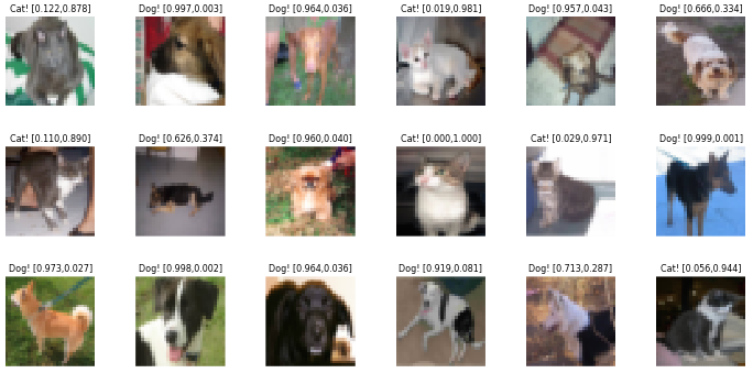
Here are the results from the best neural network (the 97.74% accuracy one) using images from the test set (the 25% randomly chosen images from the directory train):

UPDATE (11/02/2017): I was not normalizing the images before sending them to the network! I was reading again this post to start the Part 1½ when I realized the outputs were always saturating (1 or 0) and then I noticed the problem with the lack of normalization.

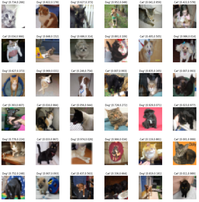
And using images never seen before (directory test1):

Ok, let’s see what we have achieved so far:

• Convince ourselves learning Keras is a nice investment!
• Create our very own first deep neural network (ok, not that deep) applying it to a well known task.
• Show off by modifying the previous example using a convolutional layer.
• Enjoy our time because when you work on something you like, it is not work anymore!

As promised, here you can visualize (or download) a Jupyter (IPython) notebook with all the source code and something else.

In the next post, we will see how to convert our simple deep neural network to a convolutional neural network. Cheers!

UPDATE (15/02/2017): Part 1½ is available here.