Easy-peasy Deep Learning and Convolutional Networks with Keras - Part 2

This is the continuation (finally!), or the Part 2, of the “Easy-peasy Deep Learning and Convolutional Networks with Keras”. This post should be something self-contained, but you may enjoy reading Part 1 and Part 1½… it’s up to you.

Around one week ago, I’d attended a CUDA workshop presented (or should I say conducted?) by my friend Anthony Morse and I’m still astounded by DIGITS. So, during the workshop, I had some interesting ideas to use on this post!

The first thing I thought when I read (or heard?) for the first time the name Convolutional Neural Network was a bunch of filters (Gimp would agree with me). I’m an Electrical Engineer and, for most of us (Electrical Engineers), convolutions start as nightmares and, gradually, become our almighty super weapon after a module like Signal and Systems.

Let’s start with something easy… a video! Below, you can observe, step-by-step, what happens when a 2D convolution (think about a filter that detects, or enhances, edges) is applied to an image:

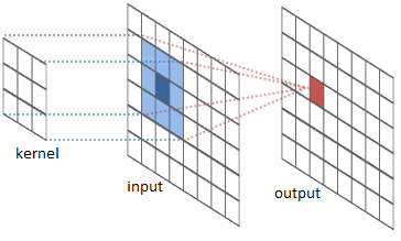
The red’ish 3x3 square moving around the cat’s face is where the kernel (an edged detector) is instantaneously applied. If the terms I’m using here are giving you goosebumps, try to read this first deep learning glossary first. When I say applied I mean an elementwise multiplication where the result is presented at the bottom (small square, really pixelated or 3x3 if you prefer). The picture, on the right hand side, is the sum of the values (you can visualize them on the small square figure at the bottom) at that instant (but the scales now are different, final result uses absolute values). If you, like me, thinks my explanation above is very poor and you want to understand what is really happening (e.g. Why does the original image have a black border?), I would suggest you to have a look on these websites: CS231n, Colah’s and Intel Labs’ River Trail project. The figure below, taken from Intel’s website, is (IMHO) the killer explanation:

Nevertheless, this post is supposed to be easy-peasy® style and I will not change it now. My definition for convolution is: a close relative of cross-correlation (pay attention to τ and t if you decide to follow the previous link and have a closer look at the initial animation I’ve presented) and very good friend of dot product (try to flatten things and it will be easier to spot it) - even the symbols have a strong resemblance. Improving even further my easy-peasy® description, another way to describe what a convolution is would be by saying it is like rubbing one function (our kernel) against another one and taking note of the result while you do it .

I’m starting to hate this idea of having this outline thing… but I will try to keep using it! If I got it right, after reading (writing, in my situation) everything and trying to figure out where all things came from and why, we should be able to:

• Undoubtedly convince ourselves Keras is cool!
• Create our first very own Convolutional Neural Network.
• Understand there’s no magic! (but if we just had enough monkeys…)
• Get a job on Facebook… ok, we will need a lot more to impress Monsieur Lecun, but this is a starting point .
• And, finally, enjoy our time while doing all the above things!

Ok, ok, ok… let’s get back to Keras and our precious Convolutional Neural Networks (aka CNNs) .

Do you remember I said CNNs were just a bunch of filters? I was not lying or making fun of you. CNNs are a mixture between a fancy filter bank and Feedforward Neural Networks, but everything works together with the help of our friend backpropagation. Recalling from Part 1, our network was initially designed only using Kera’s Dense layers:

# Just creates our Keras Sequential model
model = Sequential()

# The first layer will have a uniform initialization
model.add(Dense(768, input_dim=3072, init="uniform"))
# The ReLU 'thing' :)
model.add(Activation('relu'))

# Now this layer will have output dimension of 384
model.add(Dense(384, init="uniform"))
model.add(Activation('relu'))

# Because we want to classify between only two classes (binary), the final output is 2
model.add(Dense(2))
model.add(Activation("softmax"))

And what is the problem with the classical layers? Theoretically, none. One could, somehow, train a network with enough data to do the job. However, backpropagation is not so powerful and it would probably demand networks a lot bigger (this is my TL;DR explanation, so go and use your inner google-fu if you are not satisfied ).

CNNs are, IMHO, the engineer’s approach! They are useful because they can generate (filter out) nice features from its inputs making the life easier for Dense layers after that. Do you remember the last post of our easy-peasy® series? Ok, I would not expect anybody to fully remember anything, but that post was created because I realized visualization of internal layers was super important and I will bring back one important figure from there:

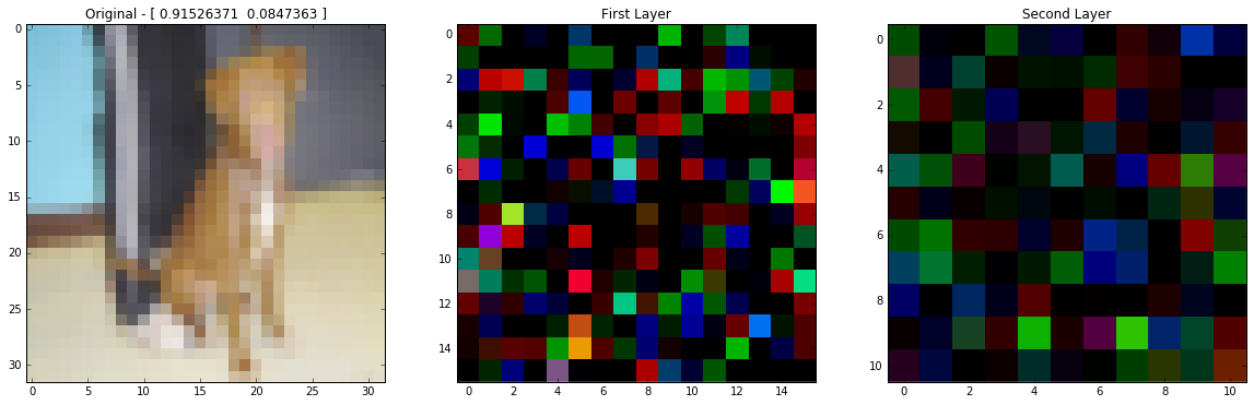
The first image is clearly a dog, but the second image (composed by the output from the first layer) is totally crazy and doesn’t look like having features to distinguish dogs from cats! So, the important bit is that I (or maybe a dense layer too) can’t even find any tiny visual clue from that image that would suggest there was a dog as input. That doesn’t mean there are no distinguishable features, but the features are hard to spot.

Now let’s see what happens when we use a convolutional layer:

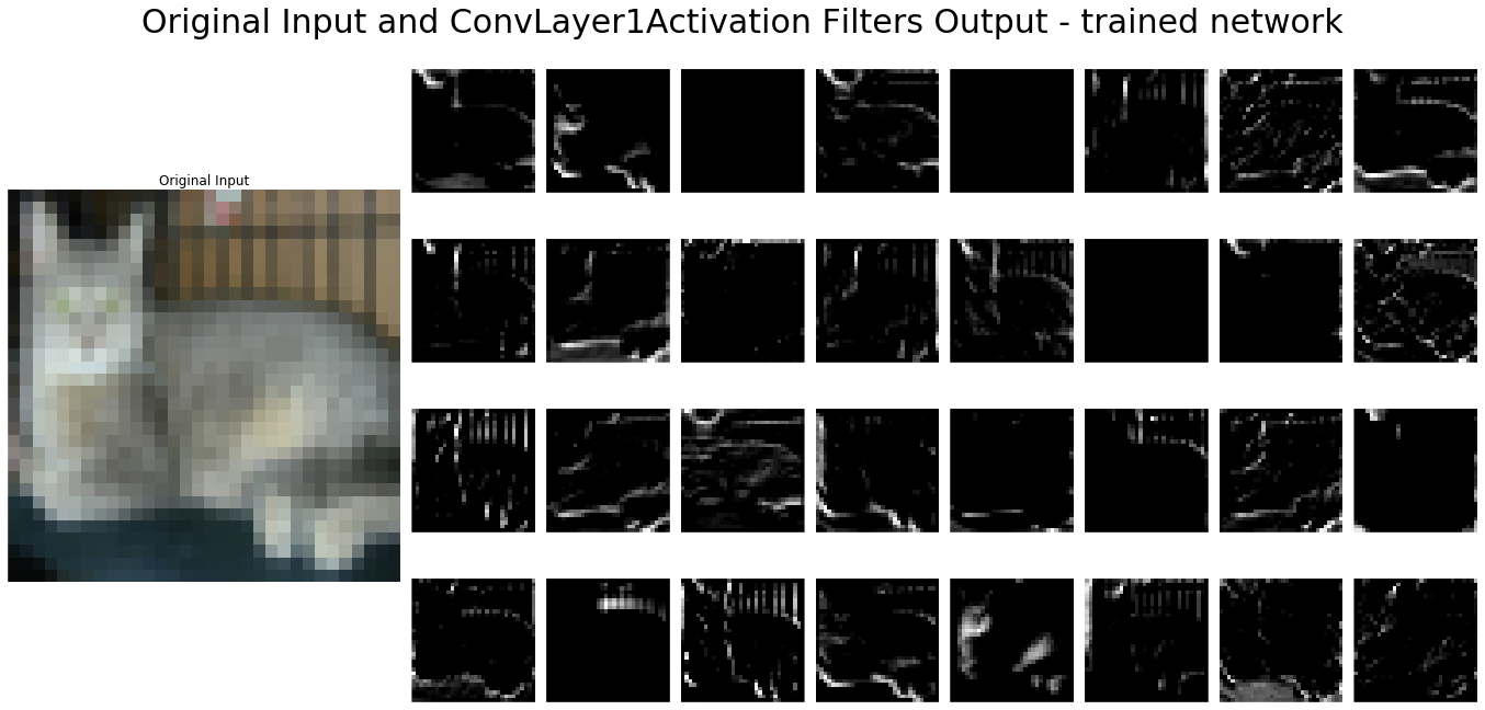
Probably, the first thing I would notice here is the number of images after the first layer. Our convolutional layer created 32, different, filtered versions of its input! Kind of cheating…

In order to have the above result, we need to replace, in our old model, the first Dense layer with a Convolution2D one:

model.add(Convolution2D(number_of_filters,
                        kernel_size[0],
                        kernel_size[1],
                        border_mode='same',
                        input_shape=input_layer_shape,
                        name='ConvLayer1'))

Where:

number_of_filters=32
kernel_size=(3,3)

This layer is composed by 32 filters (that is why we got 32 output images after the first layer!), each filter 3x3x3 (remember our input images are colorful RGB ones, therefore they have one 3x3 matrix for each color), and it will output 32 images 32x32 because border_mode='same'. It’s crystal clear that this behaviour would lead to an explosion because the next layer would always be 32x bigger than the previous… but not! If we read the Convolution2D manual, this layer receives a 4D Tensor, returns a 4D Tensor (no extra dimension created) and, consequently, no explosion at all because the generated weights do the magic of combining things for us . If we verify the shape of the weights tensor, the first convolutional layer weights tensor has shape (32, 3, 3, 3) and the second convolutional layer has shape (8, 32, 3, 3). Remember, the input image is (3, 32, 32), the first layer has 32 filters and the second only 8.

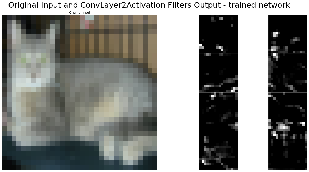
Even though the explosion problem does not afflict us, I will condense the features before the last fully-connected Keras Dense layer to speed up things by reducing the total number of weights and, therefore, calculations. The solution for this is the use of a shrinking layer and the pooling layer is what we need. From Keras, we will use a Maxpooling2d layer with pool_size=(2,2) and it will shrink our 32x32x32 output down to 32x16x16. The reduction from 32x32 to 16x16 is done by keeping the biggest value (probably that’s the reason of starting with “Max”) inside the 2x2 pool.

model.add(Convolution2D(number_of_filters,
                        kernel_size[0],
                        kernel_size[1],
                        border_mode='same',
                        input_shape=input_layer_shape,
                        name='ConvLayer2'))

model.add(Activation('relu',
                     name='ConvLayer2Activation'))

model.add(MaxPooling2D(pool_size=pool_size,
                       dim_ordering='th',
                       name='PoolingLayer2'))

Since this easy-peasy® series was not designed to beat benchmarks, but mainly to learn and understand what is happening, I will add one more set of convolutional and pooling layers. Moreover, I will reduce the number of filters from 32 to 8. I really want to see changes on the internal weights, even if this generates overfitting, thus I’ve increased the epochs to 1000. Apart from the things I’ve explained here so far, everything else will be kept the same as the Part 1 and Part 1½ posts.

Testing our new CNN against the test set (the 25% randomly chosen images from the directory train) returned us a accuracy of… 97%! You can find the saved model here.

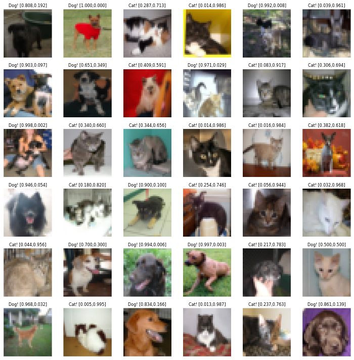
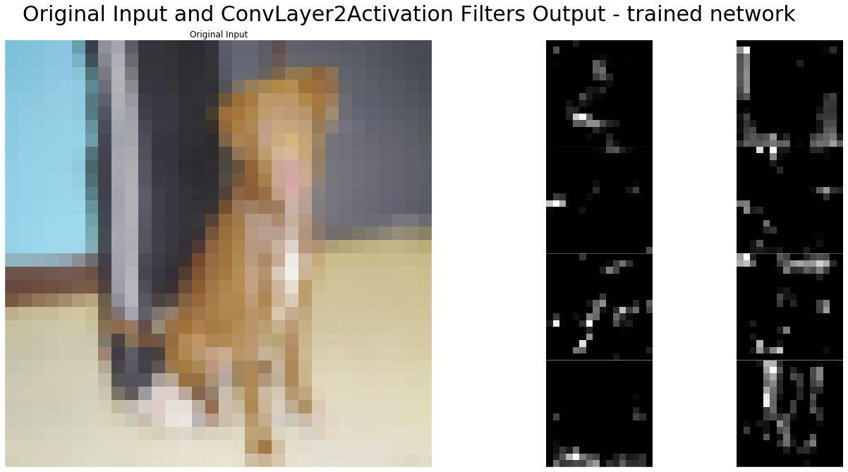
And below you can see what appears inside the CNN with the dog:

In order to help us verify the differences between dogs and cats, here are the images where a cat was the input:

After all that, I was not 100% sure if Keras was really doing convolution or cross-correlation. Instead of searching for an answer, I decided to verify it myself. First, I save the trained weights:

layer_name = 'ConvLayer1'
weights_conv1 = model.get_layer(layer_name).get_weights()[0]
bias_conv1 = model.get_layer(layer_name).get_weights()[1]

layer_name = 'ConvLayer2'
weights_conv2 = model.get_layer(layer_name).get_weights()[0]
bias_conv2 = model.get_layer(layer_name).get_weights()[1]

And then I manually do the convolution (same previous dog picture) using Scipy convolve2d.

idx = 1
input_image = testData[idx]

result = []

for i in range(3):
    result.append(convolve2d(input_image[i],
                             weights_conv1[0][i],
                             mode='same',
                             boundary='fill'))
result = numpy.array(result)

Followed by the cross-correlation using Scipy correlate2d.

idx = 1
input_image = testData[idx]

result = []

for i in range(3):
    result.append(correlate2d(input_image[i],
                              weights_conv1[0][i], mode='same'))
result = numpy.array(result)

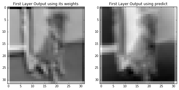
In the end I do a convolution using a cross-correlation (remember the τ and t signal change):

idx = 1
input_image = testData[idx]

result = []

for i in range(3):
    result.append(correlate2d(input_image[i],
                            numpy.fliplr(numpy.flipud(weights_conv1[0][i])), mode='same'))
result = numpy.array(result)

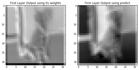
That’s it, all done!

Lastly, let’s see what we have achieved:

• Undoubtedly convince ourselves Keras is cool!
• Create our first very own Convolutional Neural Network.
• Understand there’s no magic! (but if we just had enough monkeys…)
• Get a job on Facebook… ok, we will need a lot more to impress Monsieur Lecun, but this is a starting point .
• And, finally, enjoy our time while doing all the above things!

I was almost forgetting, we can tick this box from the first post:

• Show off by modifying the previous example using a convolutional layer.

Alright, we still need to do a lot more to get that Facebook job position… but in Southern Brazil, we have a saying “Não tá morto quem peleia” that I would translate as “If you can still fight, the battle is not over” .

As promised, here you can visualize (or download) a Jupyter (IPython) notebook with all the source code and something else.

And that’s all folks! I hope you enjoyed our short Keras adventure. Cheers!