Easy-peasy Deep Learning and Convolutional Networks with Keras - Part 1½

This is the continuation, Part 1½, of the “Easy-peasy Deep Learning and Convolutional Networks with Keras”. Do you really need to read Part 1 to understand what is going on here? Honestly, probably not, but I would suggest you doing so anyway.

Before we start, let me just tell you a little bit about myself, as if you care…. Am I writing these posts to give something back to the community? Yes, this is the main reason, but I’m doing this as well because when you try to explain, or teach, something, you actually learn a lot more than just passively studying and, I would dare say, it’s even more efficient than when you are just applying your knowledge to solve a real problem. So, this is not simply an altruistic thing. However, if everybody starts behaving like this, it will naturally help all the players, therefore it’s a very very nice win-win situation in my humble opinion.

When I started writing the Part 2 post, I thought I knew a lot about deep learning convolutional networks, although, lentement, I realized there were lots and lots of things I need to understand better. That was the reason why, actually, I decided to go back to the initial model and write a Part 1½ post. To understand why convolutional layers are cool, we need to see what is happening after each layer and this can be done with Keras Dense layers too.

I’m trying to keep using this outcomes methodology, so here it comes. By the end of this post…

• Learn how images are flattened and transformed back to an image.
• Visualize what happens when we don’t put together our images in a proper way.
• Access internal layer outputs using Keras.
• Visualize the internal layer outputs as if they where images.

The first post was based on a Feedforward Neural Network and the images where rescaled (downsampling) and flattened (transformed into 1D arrays) using this bit of Python code:

 image = scipy.misc.imread(imagePath)
 new_image_size = (32,32)
 input_vector = scipy.misc.imresize(image,new_image_size).flatten()

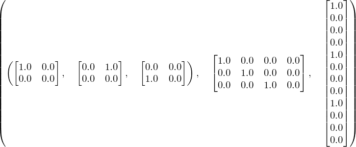
Sometimes, or most of the time, I need to think, and think again, to make sure I’m doing the right thing after I use numpy.flatten and I need to reconstruct the original array afterwards. The matrices bellow represent a simple 2x2 RBG image (I’m using Sympy Matrix and init_printing(use_latex='png') to automatically transform from numpy.ndarray to LaTeX):

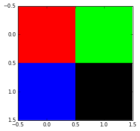
If you use matplotlib.pyplot.imshow, the result is the following image:

When we apply numpy.flatten to our initial image, the flatten method gets element (0,0) from all 3 matrices, then element (0,1)… and, at the end, just glue them together as a big 1D array.

And what does happen if you fool around with your matrices without any visual feedback? Here is a test that shows some crazy possibilities:

plt.figure(figsize=(20,10))
plt.subplot(141)
plt.imshow((testData[1].reshape(32,32,3)), interpolation='none')
plt.title("Original")
plt.subplot(142)
plt.imshow((numpy.rollaxis(testData[1].reshape(32,32,3), 1, 0)).reshape(32,32,3), interpolation='none')
plt.title("Crazy 1")
plt.subplot(143)
plt.imshow((numpy.rollaxis(testData[1].reshape(32,32,3), 2, 0)).reshape(32,32,3), interpolation='none')
plt.title("Crazy 2")
plt.subplot(144)
plt.imshow(numpy.rollaxis(testData[1].reshape(3,32,32), 0, 3), interpolation='none')
plt.title("Crazy 3")
plt.show()

The above code generates the images below:

Now, just for fun, I’m also publishing the original image, but as three matrices (I know it’s impossible to read, but it’s nice to show how even a 32x32 low-resolution image can be overwhelming when seen as matrices):

Ok, ok, I think we already had enough all those image reshaping, etc. All the discussion started to help us visualize what is happening inside our beloved neural networks. Keras has, at least, two different ways to access what is happening inside our model: functional API and creating a new model. Since, by this time, this post is sufficiently long, I will skip the functional API and stick to the new model one.

Using Keras Sequential model, we can access each layer this way:

# loads our old model
my_97perc_acc = load_model('my_97perc_acc.h5')

# creates helper variable to directly access layer instances
first_layer = my_97perc_acc.layers[0]
first_layer_after_activation = my_97perc_acc.layers[1]
second_layer = my_97perc_acc.layers[2]
second_layer_after_activation = my_97perc_acc.layers[3]

The code above loads our old model to my_97perc_acc. After that, all the layer instances are available in a list (my_97perc_acc.layers).

I want to compare our trained model to a randomly initialized one, therefore I will create another Sequential model, but this time I will give names to my layers using the argument name:

# https://keras.io/getting-started/sequential-model-guide/
# define the architecture of the network
model_rnd = Sequential()

# input layer has size "input_dim" (new_image_size[0]*new_image_size[1]*3).
# The first hidden layer will have size 768, followed by 384 and 2.
# 3072=>768=>384=>2
input_len = new_image_size[0]*new_image_size[1]*3


# A Dense layer is a fully connected NN layer (feedforward)
# https://keras.io/layers/core/#dense
# init="uniform" will initialize the weights / bias randomly
model_rnd.add(Dense(input_len/4, input_dim=input_len, init="uniform", name="Input_layer"))

# https://keras.io/layers/core/#activation
# https://keras.io/activations/
model_rnd.add(Activation('relu', name="Input_layer_act"))


# Now this layer will have output dimension of 384
model_rnd.add(Dense(input_len/8, init="uniform", name="Hidden_layer"))

model_rnd.add(Activation('relu', name="Hidden_layer_act"))

# Because we want to classify between only two classes (binary), the final output is 2
model_rnd.add(Dense(2))
model_rnd.add(Activation("softmax"))

Moreover, we can give the same layer names to the model we loaded before changing the attribute name:

first_layer.name = "Input_layer"
first_layer_after_activation.name = "Input_layer_act"
second_layer.name = "Hidden_layer"
second_layer_after_activation.name = "Hidden_layer_act"

Using same names it is super easy to swap models and, finally, we can use Keras Model to access internal layers:

model = model_rnd

# model = my_97perc_acc

layer_name = 'Input_layer_act'
input_layer_out = Model(input=model.input, output=model.get_layer(layer_name).output)

layer_name = 'Hidden_layer_act'
hidden_layer_out = Model(input=model.input, output=model.get_layer(layer_name).output)

Our intermediate outputs can be generated by simply calling the predict method:

idx = 1
input_image = testData[idx]
first_output = input_layer_out.predict(input_image.reshape(1,testData[idx].shape[0]))
second_output = hidden_layer_out.predict(input_image.reshape(1,testData[idx].shape[0]))
second_output.resize(11*11*3) # little trick to fit into a RGB image
final_output =  model.predict(input_image.reshape(1,input_image.shape[0]))

Have you noticed there’s no call to compile? Apparently, since Keras version 1.0.3 this is not necessary anymore if you just want to use predict without any training.

The resultant images can be visualized like this:

plt.figure(figsize=(20,10))
plt.subplot(131)
plt.imshow((input_image.reshape(32,32,3)), interpolation='none')
plt.title("Original - "+str(final_output[0]))
plt.subplot(132)
plt.imshow(first_output.reshape(16,16,3),interpolation='none')
plt.title("First Layer")
plt.subplot(133)
plt.imshow(second_output.reshape(11,11,3),interpolation='none')
plt.title("Second Layer")
plt.show()

Below, you can see the output for the trained network (the final output is presented in the original’s image title [P(dog),P(cat)]):

And the output for the randomly initialized one:

I think it’s important to recall here the fact that Keras Dense layer is a fully connected one. Consequently, each pixel in the image labeled First Layer receives inputs from ALL pixels in the original image (the individual pixels are multiplied by a weight, summed, added a bias and have to pass through the activation function) such situation also applies to the Second Layer in relation to the First Layer and, finally, to the last layer (our classifier) at the end. The operation used here to transform two input matrices (represented by pixel values and weights) into a scalar value (the number added to the bias before passing through the activation function) has a fancy name: dot product. This will be useful in the future….

Last, but not least: can you see patterns for dogs or cats in the First or Second Layers? I can’t .

I hope, by now, we can tick the boxes below:

• Learn how images are flattened and transformed back to an image.
• Visualize what happens when we don’t put together our images in a proper way.
• Access internal layer outputs using Keras.
• Visualize the internal layer outputs as if they where images.

As promised, here you can visualize (or download) a Jupyter (IPython) notebook with all the source code and something else .

In the next post, we will are going to see how to convert our simple deep neural network to a convolutional neural network. Cheers!